Problems: Linear Regression#
Get this problem set
Download everything (Topic1.3-Linear_Regression_Problems.zip) — the notebook and
methanol_IR.csv, in a folder that is ready to run as-is.
The Download badge at the top of the page will also give you the notebook on its own. On Vocareum everything is already set up for you.
Before you start
This problem set accompanies Linear Regression. It is worth 100 points:
Part A — Skill Checks (30 pts) — short answers, auto-graded, resubmit as often as you like until they pass.
Part B — Visualization (35 pts) — plots plus written interpretation, peer graded.
Part C — Open Ended (35 pts) — one synthesis problem, peer graded.
The parts build on each other: Part A works out the syntax you need for Part B, and Part B produces the evidence you argue from in Part C. Do them in order.
Setup#
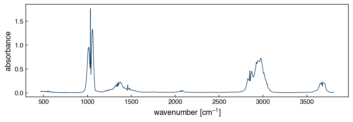
The chapter fit basis functions to an ethanol infrared spectrum. Here you will work with a methanol spectrum measured under different conditions: gas phase, 70 mmHg of methanol in nitrogen to 600 mmHg total, 5 cm path length, 2 cm⁻¹ resolution. It comes from the Coblentz Society collection in the NIST Chemistry WebBook (spectrum 8791, measured at Dow Chemical in 1964), converted from transmittance to absorbance by \(A = -\log_{10} T\).
Methanol is the simplest alcohol, so its spectrum is a stripped-down version of ethanol’s: a strong C–O stretch near 1030 cm⁻¹ and a cluster of C–H stretches between 2800 and 3050 cm⁻¹, without ethanol’s extra methylene modes. That makes it a good place to ask how many basis functions a band actually needs.
%matplotlib inline
import numpy as np
import pandas as pd
import matplotlib.pyplot as plt
try:
    plt.style.use('../settings/plot_style.mplstyle')   # available inside the book
except OSError:
    pass                                              # downloaded notebook: use defaults

df = pd.read_csv('data/methanol_IR.csv')
x_all = df['wavenumber [cm^-1]'].values
y_all = df['absorbance'].values
print(f"{len(x_all)} points, {x_all.min():.1f}-{x_all.max():.1f} cm^-1")
3567 points, 463.4-3806.6 cm^-1
fig, ax = plt.subplots(figsize=(8, 3))
ax.plot(x_all, y_all, lw=0.8)
ax.set_xlabel('wavenumber [cm$^{-1}$]')
ax.set_ylabel('absorbance');
Run this once to load the autograder. It will not run inside the book — use the downloaded notebook.
import otter
grader = otter.Notebook()
Part A — Skill Checks (30 pts)#
Three questions, 10 points each. Each asks you to assign a single number to a named variable. Run the check cell after each one; there is no limit on attempts.
A1. Locate the C–O stretch (10 pts)#
Exercise 142
Restrict the spectrum to the window \(950 \le \tilde\nu \le 1120\) cm⁻¹, which is the region every part of this problem set works in. Find the wavenumber at which absorbance is largest in that window.
Two NumPy tools you need here. A boolean array built by comparing an array against a
value can be used to index it, so band = (x_all >= 950) & (x_all <= 1120) and then
x_all[band] selects the window. And np.argmax returns the index of the largest
element, which you can use to look up the corresponding wavenumber.
Assign the wavenumber in cm⁻¹ to peak_wavenumber.
# YOUR CODE HERE
peak_wavenumber = ...
grader.check("q1")
A2. Fit one Gaussian to the band (10 pts)#
Exercise 143
Model the same window as a single Gaussian sitting on a flat baseline:
with the center \(c\) fixed at your answer from A1 and \(\sigma = 25\) cm⁻¹ (the same width
the chapter used). Build the two-column design matrix \(\bar{\bar{X}}\) — one column for the
Gaussian, one of ones for the baseline — and solve the normal equations
\(\bar{\bar{X}}^T\bar{\bar{X}}\vec{w} = \bar{\bar{X}}^T\vec{y}\) with np.linalg.solve.
Assign the Gaussian coefficient \(w_0\) to w_gauss.
# YOUR CODE HERE
w_gauss = ...
grader.check("q2")
A3. Score the fit (10 pts)#
Exercise 144
Score the A2 fit over the same window with the sum of squared errors the chapter uses:
Assign it to sse_single.
For scale: predicting nothing but the mean absorbance gives SSE = 33.35, so that is the number to beat.
# YOUR CODE HERE
sse_single = ...
grader.check("q3")
Part B — Visualization (35 pts)#
Exercise 145
One Gaussian left SSE at 11.8. Stay in the same 950–1120 cm⁻¹ window and find out what
it takes to do better, using the two basis families from the chapter. Everything here is an
ordinary linear least-squares fit: build \(\bar{\bar{X}}\), then solve
\(\bar{\bar{X}}^T\bar{\bar{X}}\vec{w} = \bar{\bar{X}}^T\vec{y}\) with np.linalg.solve.
1. Polynomials, and why the origin matters. Use the chapter’s vandermonde(x, order)
for order = 3, 5, 7, 9, 11, 13 columns, twice over:
once on the raw wavenumbers, and
once on centered wavenumbers,
x_band - x_band.mean().
For each fit record the SSE and the condition number of \(\bar{\bar{X}}^T\bar{\bar{X}}\)
(np.linalg.cond, from Linear Algebra).
The two versions describe the same family of curves — centering only moves the origin — so
any difference between them is not about the model.
2. Gaussians, placed by hand. Extend the chapter’s two-column construction: allocate
np.zeros((len(x_band), N + 1)), fill column \(j\) with a Gaussian of your chosen center
\(c_j\) and width \(\sigma_j\), and make the last column ones for the baseline. Only the
amplitudes come from the solve — the centers and widths are yours to choose.
Work from N = 1 to N = 6. For each N, move and widen the Gaussians by eye until the
fit tracks the data as well as you can get it, then record SSE and the condition number.
Say in one line what you were trying to capture with each new component.
3. Plot. The data with your N = 1, N = 3 and N = 6 fits overlaid, and beneath it,
on shared x-axes, the differences \(y - \hat{y}\) for those three.
4. Interpret, in 4–6 sentences:
Raw-wavenumber polynomials stop improving past about 7 columns, while centered ones keep improving. Explain this using your condition numbers. What is a condition number of \(10^{40}\) telling you about the weights that came back?
The Gaussian condition numbers stay below about 40 no matter how many components you add, which is some thirty orders of magnitude better. What is different about those columns?
Your Gaussian SSE should drop sharply somewhere and then nearly stop. Where, and what does that say about the band?
Label your axes with units.
# YOUR CODE HERE
fig, ax = plt.subplots()
Part C — Open Ended (35 pts)#
So far every basis function has been a Gaussian. That was a choice, not a necessity — the general linear model works with any fixed set of columns, and a different column shape may describe the same data with fewer of them.
A widely used alternative is the Voigt profile. Where a Gaussian falls off as \(e^{-x^2}\), the Voigt profile decays much more slowly away from its center, so it has noticeably heavier tails for the same central width. It is controlled by two width parameters instead of one: \(\sigma\) sets the Gaussian-like core and \(\gamma\) sets how heavy the tails are, with \(\gamma = 0\) recovering a Gaussian exactly. Use this helper:
from scipy.special import voigt_profile

def voigt(x, center, sigma, gamma):
    """One Voigt profile. gamma = 0 gives a Gaussian; larger gamma gives heavier tails."""
    return voigt_profile(x - center, sigma, gamma)
The important point for this course is that nothing about the fitting changes. Fix each center, \(\sigma\) and \(\gamma\) by hand as you did in Part B, put one profile in each column of \(\bar{\bar{X}}\), and the amplitudes are still the solution of the same normal equations. The shape parameters are chosen, not fitted.
Exercise 146
Use a Voigt basis on the same 950–1120 cm⁻¹ window to answer the question this problem set has been building toward:
How many distinct components does this band contain?
Support your answer with:
Voigt fits for
N = 1, 2, 3and at least one largerN, each with hand-chosen centers, \(\sigma\) and \(\gamma\), reporting SSE and the condition number. Compare against your Part B Gaussian results at the sameN.The fitted amplitudes of your best model. They are not all alike, and the pattern matters more than the individual values.
Evidence that your chosen
Nis not merely the largest you tried: show what one more component buys, and show the difference plot \(y - \hat{y}\) has no obvious structure left.A short written argument (one paragraph). “Number of components” can mean the number of visible maxima, or the number of columns the data actually justifies, or the number of underlying physical features. These need not be the same number, and saying so with evidence is a better answer than picking one.
Note
Domain knowledge of spectroscopy may be helpful here, but it is not required — the question can be answered entirely from the fits, the SSE and the difference plots. If you do know some spectroscopy, say what it adds; if you do not, do not go looking for it.
There is more than one defensible answer. You are graded on the reasoning and the evidence.
# YOUR CODE HERE
Summary#
Part A built a two-column design matrix by hand and solved the normal equations, exactly as the chapter does, and scored the result with the sum of squared errors: 11.8 against a mean-only baseline of 33.3.
Part B set polynomial and Gaussian bases against each other on the same band. Polynomials on raw wavenumbers stall once the condition number passes what double precision can carry; centering the same model recovers thirty orders of magnitude of conditioning. A localized Gaussian basis stays well conditioned at any size, and its SSE stops improving once there is one component per resolved maximum.
Part C changed the shape of the basis functions rather than their number, and found that three Voigt profiles describe the band better than thirteen polynomial columns or six Gaussians — then asked what “three components” actually means.
Additional Reading#
NIST Chemistry WebBook, SRD 69 — methanol IR spectrum, Coblentz Society collection no. 8791.
numpy.linalg.cond— the diagnostic behind Part B’s raw-versus-centered comparison.scipy.special.voigt_profile, used here only to evaluate a fixed shape.