Neural Network Basics

Learning Objectives

By the end of this chapter, you will be able to:

• Explain why linear and kernel methods fall short for some problems and motivate the need for neural networks.

• Describe the computation performed by a single neuron (weighted sum + activation) and implement it from scratch.

• Compare step, sigmoid, and ReLU activation functions and explain why nonlinearity is essential for learning complex functions.

• Describe the architecture of a multi-layer perceptron (MLP) and explain the universal approximation theorem conceptually.

• Derive the chain rule for a two-layer network and explain how backpropagation distributes credit across layers.

• Fit sklearn.neural_network.MLPRegressor to a regression task, visualize the training loss curve, and tune hidden-layer size to control overfitting.

%matplotlib inline
import numpy as np
import pandas as pd
import matplotlib.pyplot as plt
from sklearn.preprocessing import StandardScaler
from sklearn.model_selection import train_test_split

plt.style.use('../settings/plot_style.mplstyle')

clrs = np.array(['#003057', '#EAAA00', '#4B8B9B', '#B3A369', '#377117',
                 '#1879DB', '#8E8B76', '#F5D580', '#002233'])

Motivation: Where Simpler Methods Fall Short

The methods we have studied so far follow a common pattern: transform the raw features into a new space, then apply a linear model. Kernel methods (KRR, SVM) achieve nonlinearity by computing pairwise similarities; polynomial and symbolic regression achieve it by constructing explicit products and powers of input features.

Both approaches have fundamental limitations:

• Kernel methods scale quadratically or cubically in the number of training points. A 50,000-point dataset requires a 50,000 × 50,000 kernel matrix — impractical.

• Polynomial/symbolic regression requires explicit feature construction that grows combinatorially with input dimension and polynomial degree.

• Neither approach learns a hierarchical representation: a face recognition model should learn edges first, then corners, then parts, then faces — not a flat transformation of raw pixel values.

Neural networks address all three limitations. They learn layered feature representations directly from data, with computational cost that scales linearly in the number of training samples at inference time.

The classic motivating example is the XOR function: two inputs \(x_1, x_2 \in \{0,1\}\), output 1 if exactly one input is 1, else 0. No linear model can separate the two classes because they are not linearly separable in the original 2-D space — but a two-layer network can.

Exercise 124

Verify that no linear model can solve XOR.

1. Fit LinearRegression to X_xor and y_xor and round the predictions to 0 or 1. Report the accuracy.

2. Fit SVC(kernel='linear') and SVC(kernel='rbf'). Report accuracy for both.

3. Explain in one sentence why the RBF kernel SVC can solve XOR while a linear model cannot.

# XOR: linear model fails, MLP succeeds
from sklearn.svm import SVC
from sklearn.neural_network import MLPClassifier

X_xor = np.array([[0,0],[0,1],[1,0],[1,1]])
y_xor = np.array([0, 1, 1, 0])

linear_svm = SVC(kernel='linear').fit(X_xor, y_xor)
mlp = MLPClassifier(hidden_layer_sizes=(4,), activation='relu', max_iter=5000,
                    random_state=0).fit(X_xor, y_xor)

print(f'Linear SVM accuracy:  {linear_svm.score(X_xor, y_xor):.2f}')
print(f'MLP accuracy:         {mlp.score(X_xor, y_xor):.2f}')

Linear SVM accuracy:  0.50
MLP accuracy:         1.00

---

The Perceptron: A Single Neuron

Computation

The fundamental unit of a neural network is the neuron (or perceptron). It:

1. Takes a vector of inputs \(\mathbf{x} = [x_1, \ldots, x_n]\).

2. Computes a weighted sum: \(z = \mathbf{w}^\top \mathbf{x} + b\).

3. Passes it through a nonlinear activation function: \(a = \sigma(z)\).

def neuron(x, w, b, activation):
    z = np.dot(w, x) + b
    return activation(z)

# Step function (original perceptron)
step = lambda z: (z >= 0).astype(float)
# Sigmoid
sigmoid = lambda z: 1 / (1 + np.exp(-z))
# ReLU
relu = lambda z: np.maximum(0, z)

# Example: 2-input neuron with w = [1, -1], b = 0
w = np.array([1.0, -1.0])
b = 0.0
x_test = np.array([2.0, 1.0])
for name, fn in [('step', step), ('sigmoid', sigmoid), ('relu', relu)]:
    print(f'{name:8s}: z = {np.dot(w, x_test)+b:.2f},  a = {neuron(x_test, w, b, fn):.4f}')

step    : z = 1.00,  a = 1.0000
sigmoid : z = 1.00,  a = 0.7311
relu    : z = 1.00,  a = 1.0000

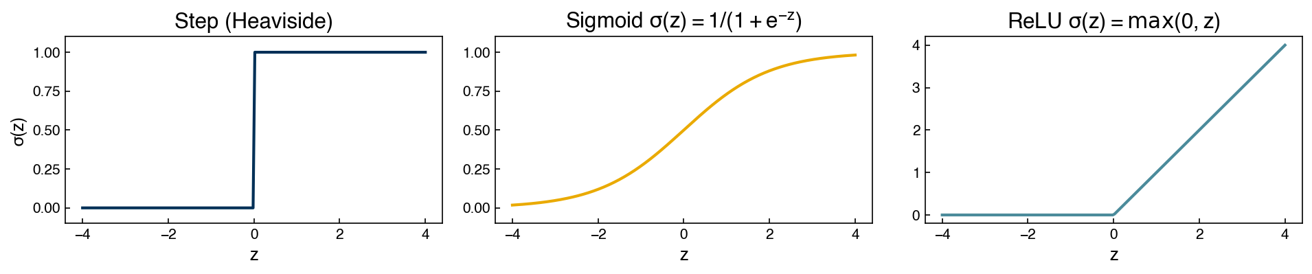
With a step activation, the neuron is a binary classifier: it fires (\(a=1\)) if the weighted sum is positive. With sigmoid or ReLU, the output is a smooth function that can represent graded responses.

Visualizing the Linear Decision Boundary

A single neuron with a step or sigmoid activation places a linear decision boundary in the input space — exactly the same as logistic regression:

xx, yy = np.meshgrid(np.linspace(-1.5, 2.5, 200), np.linspace(-1.5, 2.5, 200))
Z = np.dot(np.column_stack([xx.ravel(), yy.ravel()]),
           np.array([1.0, -1.0])) + 0.0   # z = x1 - x2
Z_sig = sigmoid(Z).reshape(xx.shape)

fig, ax = plt.subplots(figsize=(5.5, 4.5))
c = ax.contourf(xx, yy, Z_sig, levels=20, cmap='RdBu_r', alpha=0.7)
ax.contour(xx, yy, Z_sig, levels=[0.5], colors='k', linewidths=1.5)
fig.colorbar(c, ax=ax, label='σ(z)')
ax.scatter(X_xor[:, 0], X_xor[:, 1], c=[clrs[yi] for yi in y_xor],
           edgecolors='k', s=120, zorder=5)
ax.set_title('Single neuron: sigmoid output surface (XOR points overlaid)')
ax.set_xlabel('$x_1$')
ax.set_ylabel('$x_2$')
plt.tight_layout()

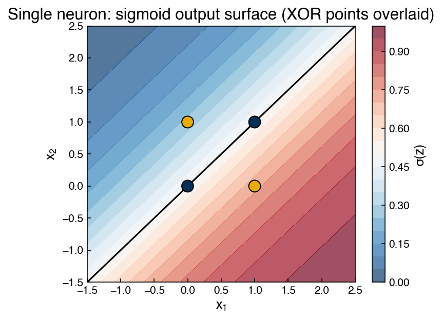
The straight black line is the decision boundary \(z = 0\) (i.e., \(x_1 - x_2 = 0\)). The four XOR points are overlaid, colored by class, and the problem is easy to see: this particular boundary puts the two same-class gold points on opposite sides, and no rotation or shift of a single straight line can isolate the two gold corners from the two navy ones. A single neuron can only draw one straight line, so it cannot solve XOR.

Exercise 125

Implement and test a single neuron from scratch.

1. Using the neuron function defined above, create a neuron with weights w = [2.0, -1.5] and bias b = 0.5. Evaluate it on all four XOR inputs using the sigmoid activation. Report the four outputs.

2. Find weights and bias by hand (not by training) such that the neuron correctly classifies the AND function: output 1 only when both inputs are 1. Verify your solution by evaluating on all four inputs.

3. Is it possible to solve XOR with a single neuron and any choice of weights? Explain why or why not.

---

Activation Functions

Why Nonlinearity Is Essential

If every neuron used a linear activation, stacking layers would still produce a linear function: \(W_2 (W_1 \mathbf{x} + \mathbf{b}_1) + \mathbf{b}_2 = (W_2 W_1)\mathbf{x} + \mathbf{b}'\) is just another linear transformation. Nonlinear activations are what allow multiple layers to represent exponentially more complex functions.

z = np.linspace(-4, 4, 200)

fig, axes = plt.subplots(1, 3, figsize=(13, 3))

# Step
axes[0].plot(z, step(z), color=clrs[0])
axes[0].set_title('Step (Heaviside)')
axes[0].set_ylim(-0.1, 1.1)
axes[0].set_xlabel('z')
axes[0].set_ylabel('σ(z)')

# Sigmoid
axes[1].plot(z, sigmoid(z), color=clrs[1])
axes[1].set_title('Sigmoid $σ(z) = 1/(1+e^{-z})$')
axes[1].set_ylim(-0.1, 1.1)
axes[1].set_xlabel('z')

# ReLU
axes[2].plot(z, relu(z), color=clrs[2])
axes[2].set_title('ReLU $σ(z) = \\max(0, z)$')
axes[2].set_xlabel('z')

plt.tight_layout()

Activation	Range	Advantages	Disadvantages
Step	\(\{0,1\}\)	Interpretable; original perceptron	Non-differentiable; no gradient
Sigmoid	\((0,1)\)	Smooth; natural probability output	Vanishing gradients for large $
Tanh	\((-1,1)\)	Zero-centered	Vanishing gradients
ReLU	\([0,\infty)\)	Fast; no vanishing gradient for \(z>0\)	“Dying ReLU” for \(z < 0\)
Leaky ReLU	\((-\infty,\infty)\)	Fixes dying ReLU	One extra hyperparameter

In practice, ReLU is the default for hidden layers in most modern networks. Sigmoid and softmax are used in output layers for binary and multi-class classification respectively.

ReLU Is a Hinge Function

If you look closely at the ReLU, \(\max(0, z)\) is exactly the piecewise-linear hinge function from Non-parametric Models. There, we built a basis of hinges \(\max(0, x - x_j)\) with a knot at every data point and fit their coefficients by least squares, turning ordinary linear regression into a linear interpolator. A ReLU neuron computes \(\max(0, wx + b)\) — the same hinge, but with a slope \(w\) and a knot located at \(-b/w\). A sum of ReLU neurons is therefore a piecewise-linear function whose breakpoints and segment slopes we control. Using the Topic 2.1 machinery (fixed knots, least-squares coefficients):

x_demo = np.linspace(0, 2*np.pi, 200)
y_true = np.sin(x_demo)

knots = np.linspace(0, 2*np.pi, 8, endpoint=False)
H = np.maximum(0, x_demo[:, None] - knots[None, :])   # one ReLU hinge per knot
H = np.column_stack([np.ones_like(x_demo), H])        # plus an intercept

coefs, *_ = np.linalg.lstsq(H, y_true, rcond=None)
y_hinge = H @ coefs

fig, ax = plt.subplots(figsize=(7, 3.5))
ax.plot(x_demo, y_true, label='sin(x)', color=clrs[0], alpha=0.5, linewidth=3)
ax.plot(x_demo, y_hinge, label='sum of 8 ReLU hinges', color=clrs[1])
ax.plot(knots, np.interp(knots, x_demo, y_hinge), 'o', color=clrs[1], ms=5)
ax.set_xlabel('x'); ax.set_ylabel('y')
ax.legend()
ax.set_title('A sum of ReLUs is a piecewise-linear interpolator')
plt.tight_layout()

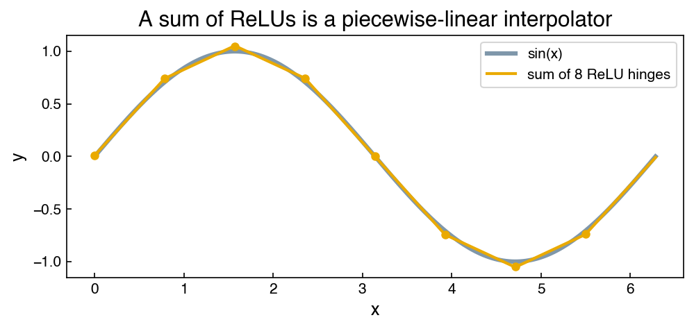
Eight hinges already trace the sine curve as eight straight segments, and adding knots makes the approximation arbitrarily good: a sum of ReLUs with different offsets and slopes is an arbitrary piecewise-linear interpolator, and piecewise-linear functions can track any continuous curve as closely as desired. The only thing a neural network adds to the Topic 2.1 picture is that the knots and slopes are not fixed in advance; they are learned by gradient descent. This is worth keeping in mind for the next section, since it is the intuition behind the universal approximation theorem.

Exercise 126

Compare the gradient properties of activation functions.

1. Plot the sigmoid, tanh, and ReLU functions over \(z \in [-4, 4]\) on the same axes.

2. Plot their derivatives (analytical or numerical) on a second set of axes.

3. For the sigmoid function, identify the range of \(z\) where the gradient falls below 0.01. What fraction of the \([-4, 4]\) range does this represent?

4. Based on your plot, explain why ReLU is preferred over sigmoid for deep networks from a gradient flow perspective.

---

Multi-Layer Perceptrons

Stacking Layers

A multi-layer perceptron (MLP) (also called a fully-connected or dense network) places many neurons side by side in a hidden layer: each neuron receives the same inputs, applies its own weights and activation, and the layer’s outputs are combined by the layer after it. The “multi-layer” in the name counts the input, hidden, and output layers — a single hidden layer of many neurons already qualifies, and it is the width of that layer (not depth) that gives the simplest MLPs their flexibility. Deeper networks chain several hidden layers, each taking the previous layer’s activations as input. The standard way to draw such a network — and the picture behind every “neural network” icon you have ever seen — is circles for neurons and lines for weights:

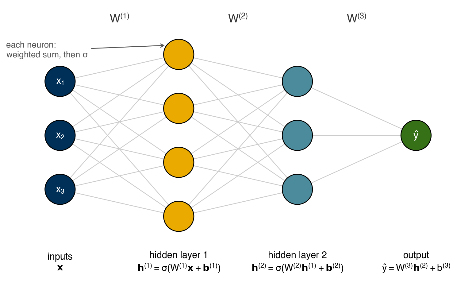
Fig. 25 A two-hidden-layer MLP (3 inputs, hidden layers of 4 and 3 neurons, 1 output). Each circle is a neuron — a weighted sum followed by an activation \(\sigma\) — and each line carries one weight. The bundle of lines connecting two columns is the weight matrix \(W^{(l)}\): one row per destination neuron, one column per source.

The math is this diagram read left to right, one column at a time:

\[\mathbf{h}^{(1)} = \sigma(W^{(1)} \mathbf{x} + \mathbf{b}^{(1)})\]

\[\mathbf{h}^{(2)} = \sigma(W^{(2)} \mathbf{h}^{(1)} + \mathbf{b}^{(2)})\]

\[\hat{y} = W^{(3)} \mathbf{h}^{(2)} + b^{(3)}\]

Each equation processes one column of the figure: collect the previous column’s values, multiply by the weights on the incoming lines (\(W^{(1)}\) is 4×3 here — four hidden neurons, each with three incoming weights), add that layer’s biases, and apply the activation. (For regression, the output layer is typically linear; for classification, softmax.)

The Universal Approximation Theorem states that a single hidden layer with enough neurons can approximate any continuous function on a compact domain. For ReLU activations you have already seen why this is plausible: one hidden layer of ReLU neurons is a sum of hinges — an arbitrary piecewise-linear interpolator that can track any continuous curve given enough knots. The theorem says nothing, however, about how many neurons are needed or how easily the model can be trained. In practice, depth (more layers) is often more efficient than width (more neurons per layer): each added layer can represent exponentially more functions for the same number of parameters.

Visualization: What the MLP’s XOR Solution Looks Like

# Fit an MLP with one hidden layer of 4 neurons to XOR and visualize its output
# surface. On a four-point dataset the full-batch quasi-Newton 'lbfgs' solver (the
# BFGS method from Numerical Optimization) is far more reliable than stochastic
# gradient descent, which frequently stalls in a flat region and never solves XOR.
mlp_xor = MLPClassifier(hidden_layer_sizes=(4,), activation='tanh',
                        solver='lbfgs', max_iter=5000, random_state=0)
mlp_xor.fit(X_xor, y_xor)
print(f'MLP accuracy on XOR: {mlp_xor.score(X_xor, y_xor):.2f}')

xx, yy = np.meshgrid(np.linspace(-0.5, 1.5, 300), np.linspace(-0.5, 1.5, 300))
P = mlp_xor.predict_proba(np.column_stack([xx.ravel(), yy.ravel()]))[:, 1].reshape(xx.shape)

fig, ax = plt.subplots(figsize=(5.5, 4.5))
c = ax.contourf(xx, yy, P, levels=20, cmap='RdBu_r', alpha=0.7)
ax.contour(xx, yy, P, levels=[0.5], colors='k', linewidths=2)
fig.colorbar(c, ax=ax, label='P(class 1)')
ax.scatter(X_xor[:, 0], X_xor[:, 1], c=[clrs[yi] for yi in y_xor],
           edgecolors='k', s=120, zorder=5)
ax.set_title('MLP output surface — XOR')
ax.set_xlabel('$x_1$')
ax.set_ylabel('$x_2$')
plt.tight_layout()

MLP accuracy on XOR: 1.00

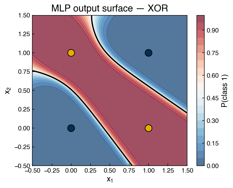
This is the same type of plot as the single-neuron surface from earlier in the chapter, but with a different model. Where the single neuron could only draw one straight line, the hidden layer’s neurons each contribute a line, and the output neuron combines them into a band: the black 0.5 contour now separates the two gold corners from the two navy ones, which no single straight line can do.

Exercise 127

Explore the effect of hidden layer width on XOR and a regression task.

1. Fit MLPClassifier with hidden_layer_sizes=(n,) for \(n \in \{1, 2, 4, 8\}\) on the XOR data. For each, report accuracy and whether the model solves XOR perfectly. What is the minimum width needed?

2. Generate a 1-D regression dataset: x = np.linspace(0, 2*np.pi, 100), y = np.sin(x) + 0.1 * np.random.randn(100). Fit MLPRegressor with one hidden layer and widths (4, 8, 16, 32, 64). Plot train and test \(r^2\) vs. width (use an 80/20 split). At what width does the model adequately fit the sine curve?

---

Training: Loss and Gradient Descent

The Loss Surface

Training a neural network means finding weights \(\{W^{(l)}, \mathbf{b}^{(l)}\}\) that minimize a loss function — which is exactly the problem of Numerical Optimization: a scalar loss, a vector of parameters, and derivatives to guide the search. Everything from that chapter transfers; what changes is the scale. For regression, the standard loss is mean squared error:

\[\mathcal{L}(\theta) = \frac{1}{n} \sum_{i=1}^{n} (y_i - \hat{y}_i(\theta))^2\]

This is the same least-squares loss we have minimized since Module 1, and it carries the same statistical meaning: Nonlinear Parameter Estimation showed that minimizing squared error is maximum likelihood estimation under the assumption of independent Gaussian noise on the targets. That assumption is a modeling choice, and other choices lead to other losses: mean absolute error corresponds to heavier-tailed noise and is less sensitive to outliers, and the cross-entropy loss used for classification is likewise a negative log-likelihood — of a Bernoulli (or categorical) model for class labels rather than a Gaussian model for continuous targets.

The loss is a function of all the weights — a surface in a very high-dimensional space. For a deep network with millions of parameters, visualizing this surface is impossible, but the key insight is that gradient descent can find a local minimum by repeatedly moving in the direction of steepest descent:

\[\theta \leftarrow \theta - \eta \nabla_\theta \mathcal{L}\]

This is precisely the update rule we implemented by hand for the Gaussian-peak problem in Topic 1.4, where the learning rate \(\eta\) (step size) posed the same dilemma: too large and the optimizer overshoots, too small and convergence is slow. The pathologies of that six-parameter problem carry over too. The loss surface is non-convex, gradients can vanish (a badly placed Gaussian there; a saturated sigmoid or dead ReLU here), and the optimizer can stall on a plateau — the failure of the default stochastic optimizer on XOR earlier in this chapter is exactly that.

Two things do change at neural-network scale:

• First-order methods take over. Topic 1.4’s workhorse BFGS builds an approximate inverse Hessian, which is practical for six parameters (and still the most reliable choice for our tiny XOR network) but not for millions. Large networks are trained with gradient-only methods, and the gradients come from automatic differentiation — Topic 1.4’s autograd, industrialized as backpropagation (next section).

• Mini-batching. Stochastic gradient descent (SGD) estimates the gradient from a random subset (mini-batch) of the data at each step. Each step is far cheaper, and the gradient noise turns out to be a feature: it helps the optimizer escape plateaus and poor local minima that would trap full-batch descent.

Exercise 128

Investigate the effect of learning rate on MLPRegressor training.

1. Using the sine regression data from the previous exercise (80/20 split, hidden_layer_sizes=(32,), random_state=0), train MLPRegressor with learning rates [1e-4, 1e-3, 1e-2, 0.1] using solver='sgd' and max_iter=200.

2. Plot the training loss curve for each learning rate on the same axes.

3. Report the final train \(r^2\) for each. Which learning rate converges fastest without diverging?

---

Training: Backpropagation

The Chain Rule on a Two-Layer Network

The challenge of training deep networks is computing \(\nabla_\theta \mathcal{L}\) efficiently — the gradient of the loss with respect to weights in the first layer depends on how those weights affect the output through all subsequent layers. Backpropagation solves this with the chain rule of calculus.

Consider a minimal two-layer network with scalar inputs and outputs:

\[z_1 = w_1 x + b_1, \quad h = \sigma(z_1)\]

\[z_2 = w_2 h + b_2, \quad \hat{y} = z_2\]

\[\mathcal{L} = (\hat{y} - y)^2\]

The gradient with respect to \(w_1\) (the first-layer weight) is:

\[\frac{\partial \mathcal{L}}{\partial w_1} = \underbrace{\frac{\partial \mathcal{L}}{\partial \hat{y}}}_{\text{output layer error}} \cdot \underbrace{\frac{\partial \hat{y}}{\partial h}}_{\text{= }w_2} \cdot \underbrace{\frac{\partial h}{\partial z_1}}_{\text{= }\sigma'(z_1)} \cdot \underbrace{\frac{\partial z_1}{\partial w_1}}_{\text{= }x}\]

In words: the output error is multiplied by the second-layer weight (how much the output depends on \(h\)), then by the activation derivative (how much \(h\) changes when \(z_1\) changes), then by the input \(x\) (how much \(z_1\) changes when \(w_1\) changes).

# Manual forward + backward pass for a one-hidden-neuron network
def forward(x, w1, b1, w2, b2):
    z1 = w1 * x + b1
    h  = sigmoid(z1)
    z2 = w2 * h + b2
    yhat = z2
    return yhat, h, z1

def backward(x, y, yhat, h, z1, w2):
    dL_dyhat = 2 * (yhat - y)           # ∂L/∂ŷ
    dyhat_dh = w2                        # ∂ŷ/∂h
    dh_dz1   = sigmoid(z1) * (1 - sigmoid(z1))   # σ' = σ(1-σ)
    dz1_dw1  = x                         # ∂z1/∂w1

    dL_dw2 = dL_dyhat * h
    dL_dw1 = dL_dyhat * dyhat_dh * dh_dz1 * dz1_dw1
    return dL_dw1, dL_dw2

# Example: one data point
x, y_true = 2.0, 1.5
w1, b1, w2, b2 = 0.5, 0.0, -0.3, 0.0

yhat, h, z1 = forward(x, w1, b1, w2, b2)
dw1, dw2 = backward(x, y_true, yhat, h, z1, w2)

print(f'Forward:  z1={z1:.4f},  h={h:.4f},  ŷ={yhat:.4f}')
print(f'Loss:     {(yhat - y_true)**2:.4f}')
print(f'∂L/∂w1 = {dw1:.6f}')
print(f'∂L/∂w2 = {dw2:.6f}')

Forward:  z1=1.0000,  h=0.7311,  ŷ=-0.2193
Loss:     2.9561
∂L/∂w1 = 0.405646
∂L/∂w2 = -2.513844

This manual calculation is exactly what PyTorch’s autograd engine performs automatically for any computational graph, regardless of depth or architecture — the key innovation that makes deep learning tractable.

Exercise 129

Verify the manual backpropagation calculation numerically.

1. Using the forward and backward functions above with x=2.0, y_true=1.5, w1=0.5, b1=0.0, w2=-0.3, b2=0.0, compute the analytical gradients dL_dw1 and dL_dw2.

2. Compute the same gradients numerically using finite differences: \(\partial L / \partial w_1 \approx [L(w_1 + h) - L(w_1 - h)] / (2h)\) with \(h = 10^{-5}\).

3. Report the absolute difference between the analytical and numerical gradients. Are they in agreement to at least 6 decimal places?

---

Demonstration: MLPRegressor on the Dow Dataset

Time to put the pieces together on a real problem: predicting the Dow impurity from the plant’s forty process sensors. We will use scikit-learn’s MLPRegressor — the simplest practical neural-network implementation. It wraps everything this chapter has covered (hidden layers, activations, mini-batch training with adam, early stopping) behind the same fit/score interface as every other sklearn model, which makes it ideal for moderate-sized tabular problems like this one. Its limitation is flexibility: custom architectures, GPUs, and non-standard training loops require a framework like PyTorch, which is exactly where Neural Network Architectures picks up.

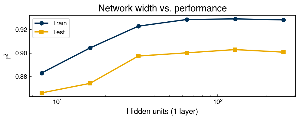
The workflow has four steps, each in its own cell below: prepare and standardize the data, fit the network, inspect the training curve, and sweep the architecture.

Fitting and Training Loss

from sklearn.neural_network import MLPRegressor

# Load and prepare Dow data
df = pd.read_excel('data/impurity_dataset-training.xlsx')

def is_real_and_finite(x):
    try:
        val = float(x)
        return np.isfinite(val)
    except (TypeError, ValueError):
        return False

nondate = df.columns[1:]
numeric_map = df[nondate].apply(lambda col: col.map(is_real_and_finite))
real_rows = numeric_map.all(axis=1).values

X_dow = df[nondate].values[real_rows, :-5].astype(float)
y_dow = df[nondate].values[real_rows, -3].astype(float)

X_train, X_test, y_train, y_test = train_test_split(
    X_dow, y_dow, test_size=0.2, random_state=0)

# Standardize
scaler = StandardScaler()
X_tr = scaler.fit_transform(X_train)
X_te = scaler.transform(X_test)

The preparation cell filters out rows with non-numeric entries (the same data-quality issue from Module 4), takes the process sensors as features and the impurity as the target, splits off a test set, and standardizes the features. Standardization is not optional for neural networks: gradient descent takes the same step size \(\eta\) in every direction, so features with very different scales produce a badly conditioned loss surface that trains slowly or not at all. (The scaler is fit on the training data only — the leakage discipline from Module 2.)

Now the fit. One hidden layer of 64 ReLU neurons, trained with adam; early_stopping holds out 10% of the training data as a validation set and stops training when the validation score stops improving — the same overfitting guard we have used since Module 2, built into the training loop:

mlp_reg = MLPRegressor(
    hidden_layer_sizes=(64,),
    activation='relu',
    solver='adam',
    max_iter=500,
    early_stopping=True,
    validation_fraction=0.1,
    random_state=0,
    verbose=False,
)
mlp_reg.fit(X_tr, y_train)

print(f'Train r²: {mlp_reg.score(X_tr, y_train):.3f}')
print(f'Test  r²: {mlp_reg.score(X_te, y_test):.3f}')
print(f'Stopped at iteration: {mlp_reg.n_iter_}')

Train r²: 0.914
Test  r²: 0.902
Stopped at iteration: 161

The train and test \(r^2\) land close together — the network generalizes — and the third line reports when early stopping fired. The word “iteration” here needs unpacking, because neural-network training has two nested loops:

• An epoch is one complete pass through the training data. Within each epoch, the data is split into mini-batches, and the weights are updated once per batch — so a single epoch contains many gradient updates (n_samples / batch_size of them).

• In scikit-learn, one “iteration” is one epoch: max_iter, n_iter_, and each point of loss_curve_ all count full passes through the data, not individual updates. Beware that other frameworks (PyTorch included) often use “iteration” for a single mini-batch update instead — when reading training logs, always check which loop is being counted.

Plotting the loss after every epoch gives the standard training diagnostic:

fig, ax = plt.subplots(figsize=(7, 3))
ax.plot(mlp_reg.loss_curve_, label='Training loss')
ax.plot(mlp_reg.validation_scores_, label='Validation r²')
ax.set_xlabel('Epoch')
ax.set_ylabel('Loss / Score')
ax.set_title('Training curve — MLPRegressor')
ax.legend()
plt.tight_layout()

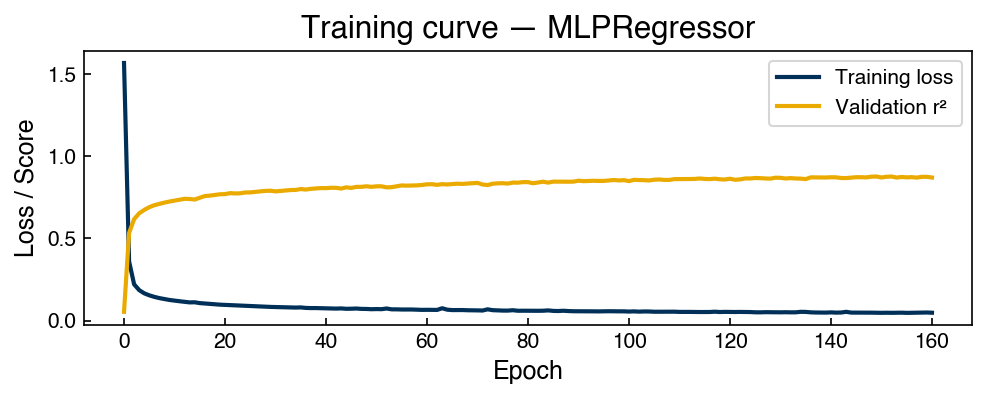
The training loss falls steeply in the first epochs and then flattens, while the validation \(r^2\) climbs and plateaus; the point where it stops improving is where early stopping ends the run. A training curve plays the same role for a neural network that a convergence check did for the optimizers of Topic 1.4: it is the first thing to check when results are unexpected.

Effect of Hidden Layer Size

sizes = [8, 16, 32, 64, 128, 256]
train_scores, test_scores = [], []

for n in sizes:
    m = MLPRegressor(hidden_layer_sizes=(n,), activation='relu', solver='adam',
                     max_iter=500, random_state=0)
    m.fit(X_tr, y_train)
    train_scores.append(m.score(X_tr, y_train))
    test_scores.append(m.score(X_te, y_test))

fig, ax = plt.subplots(figsize=(7, 3))
ax.semilogx(sizes, train_scores, 'o-', label='Train')
ax.semilogx(sizes, test_scores,  's-', label='Test')
ax.set_xlabel('Hidden units (1 layer)')
ax.set_ylabel('$r^2$')
ax.set_title('Network width vs. performance')
ax.legend()
plt.tight_layout()

As the hidden layer grows, training \(r^2\) rises at first — more capacity — but then levels off and even dips slightly at the largest widths. This may be surprising: a wider network strictly contains the smaller ones, so at the true minimum of the loss its training score could never be worse. However, that guarantee only applies at the true minimum. All of these networks share the same fixed budget (max_iter=500, one adam run from one random initialization), and the larger the network, the further from converged that budget leaves it. This is a fundamental difference from the linear models of Modules 1–2, where the least-squares solution is unique and computed in closed form: a neural network’s reported performance depends on the model and its optimization together. The architecture, optimizer, learning rate, initialization, and iteration budget all affect the numbers, and changing any of them changes the “result.” The test curve tells the more familiar story: it peaks around 64–128 units and gains nothing beyond, while the persistent train–test gap signals mild overfitting. Early stopping (early_stopping=True) helps, but is not a substitute for choosing a network architecture appropriate to the dataset size.

Exercise 130

Using the Dow dataset with X_tr, X_te, y_train, y_test from above, explore the effect of network depth.

1. Train MLPRegressor with one hidden layer of 64 units and then with two hidden layers of sizes (64, 32). Use early_stopping=True and random_state=0. Report train and test \(r^2\) for both.

2. Plot the training loss curve for each configuration on the same axes. Which converges faster?

3. Change the activation from 'relu' to 'tanh' for the two-layer network. Does it affect the test \(r^2\)?

4. From the bias-variance perspective, what does a high train \(r^2\) but low test \(r^2\) tell you about the model?

---

Hyperparameter Guide

The table below summarizes the most important hyperparameters and how to tune them:

Hyperparameter	What it controls	Practical guidance
Hidden layer sizes (depth × width)	Model capacity	Start with 1–2 layers, 32–128 units; increase only if underfitting
Activation	Nonlinearity type	Use 'relu' by default; 'tanh' for smooth outputs
Learning rate	Step size in SGD	Adam with default lr (0.001) works well; decrease if loss oscillates
Batch size	Gradient noise level	Larger batches → smoother gradients; smaller → more regularization
Early stopping	Overfitting control	Always enable for small datasets; monitor validation loss
L2 regularization (alpha)	Weight magnitude penalty	Increase if test r² << train r²

Exercise 131

Explore the effect of L2 regularization on the Dow MLPRegressor.

1. Using X_tr, X_te, y_train, y_test from above, train MLPRegressor with hidden_layer_sizes=(128,), solver='adam', max_iter=500, random_state=0, and L2 penalty alpha swept over [1e-5, 1e-4, 1e-3, 1e-2, 0.1, 1.0].

2. For each alpha, record train \(r^2\) and test \(r^2\).

3. Plot train and test \(r^2\) vs. log10(alpha). Identify the alpha that maximizes test \(r^2\) and note how the gap between train and test \(r^2\) changes.

---

Summary

• Neural networks learn layered feature representations: each layer transforms the previous layer’s activations, allowing the network to represent arbitrarily complex functions.

• A single neuron computes \(a = \sigma(\mathbf{w}^\top \mathbf{x} + b)\). Without a nonlinear activation \(\sigma\), stacking layers is equivalent to a single linear model.

• Common activations: step (non-differentiable, historical), sigmoid (smooth, vanishing gradient for large \(|z|\)), ReLU (fast, no vanishing gradient for \(z > 0\), default for hidden layers).

• Backpropagation applies the chain rule to propagate the gradient from the output back through each layer, enabling efficient computation of \(\nabla_\theta \mathcal{L}\) for any depth.

• sklearn.neural_network.MLPRegressor provides a practical interface for regression with MLPs. Training loss curves and width/depth sweeps are essential diagnostics for understanding capacity and overfitting.

Additional Reading

• Goodfellow, I., Bengio, Y. & Courville, A. (2016), Deep Learning — the standard reference, free at deeplearningbook.org

• Nielsen, M. A. (2015), Neural Networks and Deep Learning — free online book with excellent visual intuitions: neuralnetworksanddeeplearning.com

• scikit-learn User Guide: MLPRegressor, Neural network models